What Is The Total Area Under A Normal Curve
Arias News
Mar 29, 2025 · 6 min read
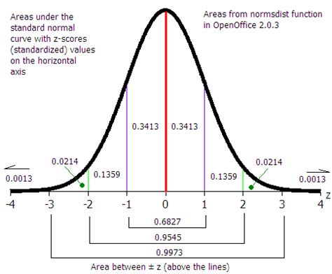
Table of Contents
What is the Total Area Under a Normal Curve?
The normal curve, also known as the Gaussian curve or bell curve, is a fundamental concept in statistics and probability. Its distinctive bell shape represents the distribution of a vast array of natural phenomena, from human heights and IQ scores to measurement errors in scientific experiments. Understanding the total area under this curve is crucial for interpreting probabilities and making inferences from data. This article delves deep into the properties of the normal curve and meticulously explains why the total area under it always equals one.
The Nature of the Normal Distribution
Before tackling the area under the curve, let's solidify our understanding of the normal distribution itself. It's characterized by two parameters:
- Mean (μ): This represents the average or central tendency of the data. It's located precisely at the peak of the bell curve.
- Standard Deviation (σ): This measures the spread or dispersion of the data. A larger standard deviation indicates a wider, flatter curve, while a smaller standard deviation results in a narrower, taller curve.
The equation defining the normal distribution is relatively complex, involving exponential and π (pi):
f(x) = (1 / (σ√(2π))) * e^(-(x-μ)² / (2σ²))
However, we don't need to delve into the intricacies of this equation to understand the total area. The key takeaway is that this equation describes a continuous probability density function.
Probability Density Functions: A Crucial Concept
A probability density function (PDF) describes the relative likelihood of a continuous random variable taking on a given value. Unlike discrete probability distributions where you can assign probabilities to individual points, the PDF assigns probabilities to intervals or ranges of values.
The crucial connection to the area under the curve lies here:
The probability that a random variable X falls within a specific interval [a, b] is equal to the area under the curve of the PDF between a and b.
This is a fundamental theorem of probability theory.
Why the Total Area Equals One
Now, let's address the central question: why does the total area under the normal curve always equal one? The reason stems directly from the properties of probability density functions:
- Total Probability: The total probability of all possible outcomes for a random variable must always sum to one (or 100%). This is axiomatic in probability theory – something must happen.
- Area Representation of Probability: As mentioned earlier, the area under the PDF represents probability.
- Normal Curve encompasses all possibilities: The normal curve extends infinitely in both directions along the x-axis (though it rapidly approaches zero). This encompasses all possible values of the random variable.
Therefore, since the area under the curve represents the probability of all possible outcomes, and the total probability must equal one, the total area under the normal curve must equal one.
Visualizing the Area: A Practical Example
Imagine you're measuring the height of adult women in a large population. Assuming height follows a normal distribution, you can plot it on a normal curve. The total area under that curve represents the probability that a randomly selected woman will have some height. Since every woman has some height, the probability of this is 100%, or 1.
The Role of Standard Deviation in Area Calculation
While the total area always remains 1, the standard deviation significantly influences the shape and distribution of that area. A larger standard deviation leads to a flatter, wider curve, spreading the probability across a larger range of values. Conversely, a smaller standard deviation results in a taller, narrower curve, concentrating the probability around the mean. However, regardless of the standard deviation, the total integrated area remains constant at 1.
Using the Normal Distribution in Practice: Z-scores and Tables
Calculating probabilities using the normal distribution's complex equation directly is challenging. This is where Z-scores and standard normal tables come in. A Z-score standardizes a data point by expressing it in terms of standard deviations from the mean:
Z = (x - μ) / σ
This converts any normal distribution into a standard normal distribution with a mean of 0 and a standard deviation of 1. Standard normal tables then provide the area (probability) under the curve to the left of a given Z-score. Since the total area is 1, you can calculate probabilities for any interval using these tables. For example, if you want to find the probability that a randomly selected value is between two values, say a and b, you would consult the table to find the area to the left of b, and then subtract the area to the left of a. The difference gives you the desired probability.
Applications of the Normal Curve and its Area
The normal distribution and its associated area calculations are ubiquitous across numerous fields:
- Quality Control: Identifying outliers and ensuring product consistency.
- Finance: Modeling asset prices and risk assessment.
- Medicine: Analyzing clinical trial data and assessing treatment effectiveness.
- Engineering: Understanding measurement errors and predicting system performance.
- Social Sciences: Studying population characteristics and conducting surveys.
The ability to calculate probabilities using the normal curve allows researchers to draw inferences, make predictions, and make informed decisions based on data.
Beyond the Standard Normal Distribution: Other Normal Distributions
While the standard normal distribution (mean = 0, standard deviation = 1) is often used for calculations due to the availability of tables, numerous other normal distributions exist with different means and standard deviations. The total area under each of these curves, however, remains unchanged: it always equals one. The difference lies in how this area is distributed along the x-axis, reflecting the specific mean and standard deviation of the distribution in question.
Approximating other distributions with the Normal Curve: The Central Limit Theorem
The normal distribution’s prevalence extends beyond its direct applications. The Central Limit Theorem (CLT) states that the distribution of sample means from any population (regardless of its original distribution) will approach a normal distribution as the sample size increases. This makes the normal distribution a powerful tool for statistical inference, even when dealing with non-normally distributed data. The CLT greatly enhances the applicability of normal curve analysis.
Conclusion: The Unifying Principle of Probability
The fact that the total area under a normal curve always equals one isn't merely a mathematical curiosity; it's a fundamental principle reflecting the very nature of probability. It reinforces the idea that the area under the curve represents probability, and the total probability of all possible outcomes must always sum to one. Understanding this concept is essential for anyone working with statistical data and interpreting the results of various analyses relying on the normal distribution. From quality control to financial modeling, the normal curve and its properties are indispensable tools in modern quantitative analysis. Mastering its applications, particularly the calculation and interpretation of areas, is paramount for anyone seeking to work within these fields.
Latest Posts
Latest Posts
-
How Many Bags Are In A Ton Of Wood Pellets
Mar 31, 2025
-
What Is The Greatest Common Factor Of 27 And 45
Mar 31, 2025
-
3 4 Cup Sugar Is How Many Grams
Mar 31, 2025
-
Did Glen Campbell Sing In The Movie Chisum
Mar 31, 2025
-
Only What You Do For Christ Will Last Scripture
Mar 31, 2025
Related Post
Thank you for visiting our website which covers about What Is The Total Area Under A Normal Curve . We hope the information provided has been useful to you. Feel free to contact us if you have any questions or need further assistance. See you next time and don't miss to bookmark.
